
 The South African
Published in RADIO BYGONES NO 111, February/March 2008
Ionosphere Recorder
During the Second World War, while serving as a technical officer responsible for radar in the Special Signals Services of the South African Corps of Signals, Wadley had given some thought to the design of continuously tunable receivers. But the first application to which he applied his ideas was not a radio receiver but was what he called an ionosphere recorder, which today we would call an ionosonde. He was then working at the Telecommunications Research Laboratory (TRL) of the South African Council for Scientific and Industriul Research, or CSIR, in Johannesburg. This article will present some technical details of that instrument and will concentrate particularly on the method Wadley used to generate a signal that swept continuously from zero to 20MHz; without the need for any band-switching.
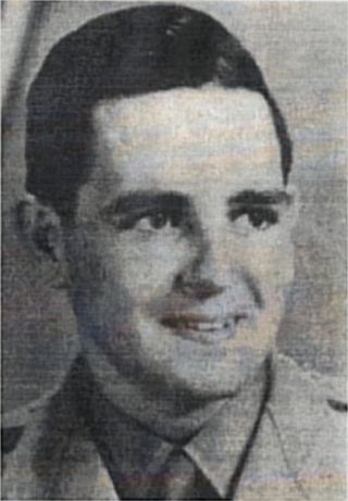
Fig. 1. Trevor Wadley photographed in uniform during the war
when he was serving in the South African Corps of Signals
Probing The Ionosphere
Two highly significant experiments were conducted late in 1924 and during the early months of the following year. The first of them went a long way towards earning the man behind it the Nobel Prize for Physics in 1947. The other, though in many ways the more important in terms of the techniques used, gained the two men responsible for it little by way of formal recognition other than the acknowledgement from generations of radar practitioners that theirs was the first demonstration of pulse radar.
Professor Sir Edward Appleton was awarded the highest of science's accolades in 1947 for his investigation of the physics of the upper atmosphere, and especially for the discovery of what became known us the Appleton Layer. The crucial experiments were carried out at Oxford University (though Appleton was working at the Cavendish Laboratory in Cambridge at the time).
It so happened that the experiment depended rather critically on the radio receiver being close enough to the BBC transmitter in Boumemouth, so that the ground wave signal was of similar strength to one that Appleton suspected was being reflected from some conducting region in space. Oxford was well placed whereas Cambridge was too far from Bournemouth to satisfy this requirement.
The technique that Appleton, and his student Miles Barnett from New Zealand, used in December 1924 required that the BBC transmitter be varied in frequency (after normal programmes had ceased for the night, of course!), such that the wavelengths of the transmitted signals would change over a brief period of time. If, as Appleton assumed would happen, two separate signals were received in Oxford whose combined strength varied during that time, then a simple calculation would indicate the height at which one of them was being reflected from some region in the atmosphere above. As history now records, that is just what did happen and a region of charged particles, which became known as the Heaviside Layer, was shown to exist at a height of about 80km.
Since the reclusive British physicist Oliver Heaviside was not the only man to have suggested, in 1902. that just such a conducting region capable of returning radio signals to earth might exist in space, but shared that distinction with American by the name of A. E. Kennelly (and one or two others before him), the reflecting layer soon became known as the Kennelly-Heaviside layer - at least in the United States.
E, F and D-Layers
Following that triumph in 1924, Appleton went on to discover another region at a height of about 250km that also had these special reflecting properties and, subsequently, it was named after him. However, it was Appleton himself who decided to call them the E and the F-Iayers, and quite soon afterwards the D-Iayer, which was somewhat lower down, and so these various regions of the ionosphere - a name given to it by Robert Watson-Watt in 1926 - were recognized as the means by which radio signals were able to travel vast distances beyond the horizon and sometimes to be absorbed within it too.
These discoveries opened up a completely new field of physics and so the understanding of the ionosphere, its constituents and how it varied with both time and space became of immense impommce to both broadcasters and to all other users of this remarkable means of long-distance wireless communications. But a detailed study of the ionosphere required special instruments and the most important of these was not based on Appleton and Barnett's experiment but rather on one carried out near Washington DC between July and September 1925.
Gregory Breit and Merle Tuve, physicists working at the Carnegie Institution in Washington, used a pulse transmitter at the Naval Research Laboratory, some 11 km from their receiver and operating at wavelengths from 41 to 71 m, to measure the height at which those pulses were being returned to earth. They did this by determining the time of flight of a given pulse as it travelled to the point of reflection and back to the receiver. Knowing the speed of light, the height of the reflecting point followed directly.
Their method was both easier to understand but, more importantly, it was easier to implement than the frequency-change technique used by Appleton and Barnett. It soon became the basis of what, since 1955, has been called an ionosonde, but in those days was known as a sounder.
Though Breit and Tuve had detected the ionosphere by means of a powerful new technique, they did not pursue this line of research but soon became absorbed in that other exciting new field: atomic physics. However, in little more than a decade, their method of using high-energy radio frequency pulses to detect and measure the distance to some reflecting object would make them amongst the earliest of the many radar pioneers.
Ionosondes and Ionograms
The first swept frequency ionospheric sounder was designed at the National Bureau of Standards in the USA in 1929, while in England the world's first programme of hourly soundiungs of the ionosphere began at the Radio Research Station in Sough, Buckinghamshire, at noon on 11 January 1931. Photographs of those early ionograms had to await the development of suitable cathode ray tubes and so the first photographic records of swept-frequency ionograms only appeared in both countries in 1933.
From then on, until the launch of artificial satellites, long-distance radio communications depended entirely on the existence of a worldwide network of ionosondes to monitor the ionosphere so that the optimum communication frequencies for a whole host of applications could be predicted.
Even by 1990, when satellite services were well established, there were 52 ionosondes in service around the world, some of which had been providing data continuously for at least two 11-year solar cycles. And by 2006, when many thought that HF radio had had its day, the number of ionosondes in use globally had actually increased to about 70.
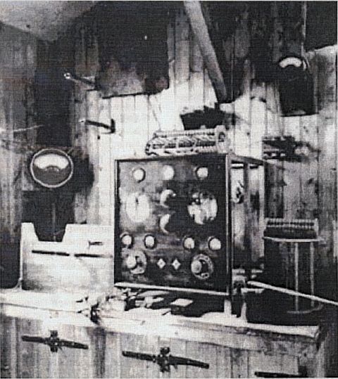
Fig. 2. The first ionosonde transmitter used at Slough in 1931.
Ionogram
The useful output from an ionosonde is called an ionogram, which is a record of a sweep across a portion of the HF spectrum showing the echoes coming back from the ionised regions immediately above the transmitting antenna. For this reason it is known as a vertical incidence ionogram and it has some very distinctive and characteristic shapes. To illustrate these I've chosen a most appropriate ionogram generated by the modern digital ionosonde at the Rutherford Appleton Laboratory at Chilton near Oxford. It was recorded at noon on 11 January 2001, the 70th anniversary of continuous ionospheric sounding in England. Since then, a mass of archived data, now all stored on computer at Chilton, represents the most complete set of continuous ionospheric records anywhere in the world.
The horizontal axis on the graph (Figure 3) gives the frequency range in megahertz covered by the sweep, while the vertical axis is the virtual height in kilometres at which reflections occur. It is called the virtual height because that is the height that would be reached by a vertically incident pulse of radio energy if it travelled consistently at the speed of light. Since the ionosphere is a complex dielectric medium the speed of propagation decreases as the pulse enters those ionised regions and so the wave slows down. The actual height at the point of reflection is therefore always somewhat less than the virtual height.
The sharp upward tilt seen on the traces does not imply that the layer suddenly increases in height but is, in fact, the clearest indication that the speed of the wave decreases sharply above a certain altitude making it appear as if the layer height increases. The splitting of the trace into two is caused by the earth's magnetic field. The frequency at which the left-hand trace (or ordinary ray) turns sharply upward is called the critical frequency and is denoted as foE, foF1 and foF2 for the E, FI and F2 layers, respectively, while that on the right, or extraordinary ray, is denoted by fxF2 and so on. The traces visible at double the altitude are the 'second bounces' of the signal between the ionosphere and the earth and do not represent yet other layers higher up.
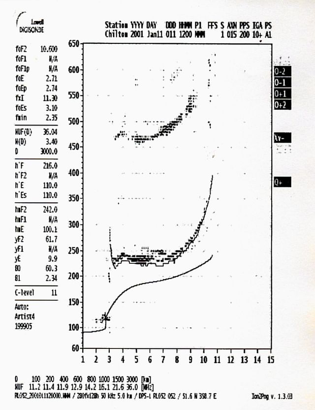
Fig. 3. A vertical incidence ionogram from the modern digital ionosonde at Chilton,
recorded on the 70th anniversary of the first such recording made in England on 11 January 1931.
The ordinary ray critical frequency (tabulated with other important parameters on the left of the chart) is a most important figure for determining the maximum usable frequency (MUF) that will propagate over a given distance when signals are reflected at that particular point in the ionosphere. A list of MUFs is shown at the foot of the graph for various transmission distances.
Genius At Work
All those who worked alongside Trevor Wadley in the Telecommunications Research Laboratory (TRL) of the South African Council for Scientific and Industrial Research (CSIR) in Johannesburg commented on the approach he adopted when tackling any new and often unusual project. He would sit at his desk for the better part of a couple of hours, usually with his eyes closed.
To those who'd not encountered him before the man was clearly having a rest - if not already fast asleep - since he was doing nothing. Then he'd reach for a pencil, find a sheet of paper, and begin to sketch furiously what soon became apparent as a block diagram, complete with much annotation. Underneath would appear various numbers, some algebra and further diagrams now in the form of electronic circuits, but never complete circuits, just those bits that were rather unusual and often incomprehensibly so to the average onlooker. Having completed that exercise, Wadley took himself off to the workbench in his laboratory and began wiring up components onto any convenient aluminium chassis that happened to be handy. That feverish constructional phase always led, in what seemed like no time at all, to a prototype that to the astonishment of his colleagues always seemed to work first time too!
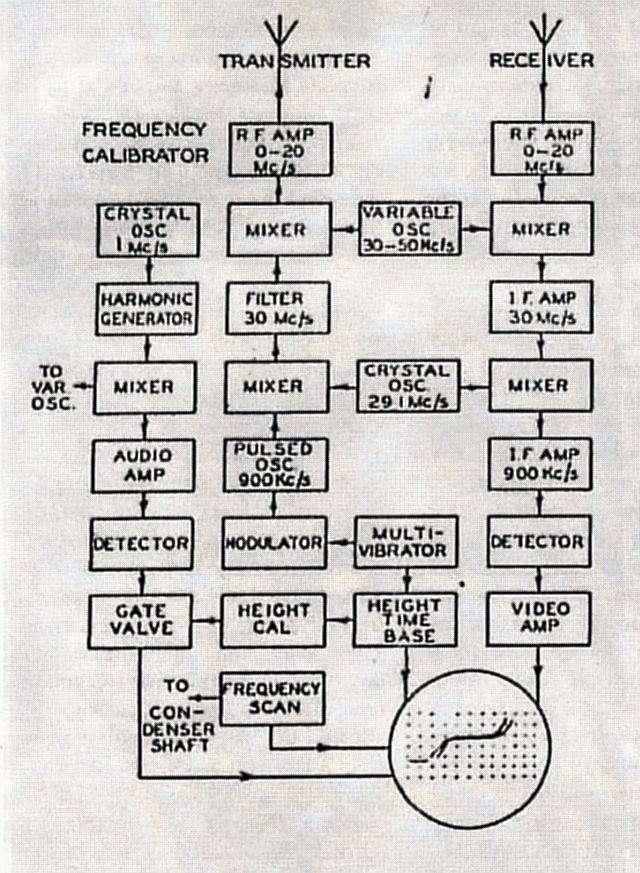
Fig. 4. Block diagram of Wadley's single-band ionosphere recorder.
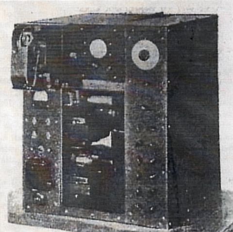
Fig. 5. A general view of the ionosonde showing the 16-mm cine camera
at the top left that photographs the long-afterglow cathode ray tube and the second one,
in the centre for monitoring the performance of the equipment.
This ability to conceive of the solution to a problem almost entirely in his head, and usually involving a most unconventional approach, marked Wadley out as an extraordinary man and as an electronics engineer of sheer brilliance. One has heard similar things said about Alan Blumlein and the remarkable F. C. (Freddie) Williams, both of the TRL's often confused near-acronym, the TRE (Telecommunications Research Establishment) in Malvern, who also exhibited many similar traits. It would seem that electronics geniuses design not on paper but in their heads. In Wadley's case paper served only as an aide-memoire afterwards.
No Bandswitch
In 1947, Wadley's ionosphere recorder was certainly most unusual when compared with the other sounders in use at that time just after the war. First of all it contained only one moving part - a motor-driven variable capacitor - that tuned the transmitter and receiver in synchronism from a few hundred kilohertz to 20MHz in about seven seconds. And there was no bandswitch in sight, which was quite unheard of in those days of superhet receivers intended to cover such a wide frequency range. What's more, the receiver kept perfectly in step with the transmitter as it swept across that spectrum thereby ensuring that any sharply tuned filters in the signal path never unwittingly attenuated or distorted the important signals reflected from the ionosphere.
Most important of all, since this instrument was intended to make accurate measurements of the critical frequencies and other characteristics of the rapidly changing ionosphere, its calibration was completely independent of the geometrical law defining the shape of the variable capacitor's plates. This meant that any capacitor of the correct value and not necessarily a high-precision unit could be used. To those schooled in the art of superhet receiver design all this sounded like heresy. But then that was almost Wadley's philosophy too!
A Single-Band Sounder
The block diagram (Figure 4, taken from Wadley's 1949 paper in the Proceedings of the IEE) shows the complete ionosonde. The first thing to notice is that it contains four oscillators: a VFO from 30 to 50MHz; two crystal-controlled oscillators at 29.1MHz and at 1 MHz; and a pulsing oscillator at 900kHz with a pulse width of about 70 microseconds. The reason for choosing 900kHz and not 1 MHz, which might seem just as appropriate, will become clear later on. The combination of all these frequencies in various mixers, and the subsequent selection of the required mixer product using suitable filters, ultimately produced a pulsed signal from the transmitter with a peak output of about 1kW. The functioning of the transmitter will be described first.
The 900kHz and 29.1 MHz signals are mixed and their sum is selected by the 30MHz bandpass filter. This signal is then mixed with the output from the VFO leading to a signal varying from zero to 20MHz that sweeps continuously across the band, as determined by the variable capacitor that was driven by an electric motor. The swept signal is then fed to a four-stage, untuned class-A amplifier, the driver for the power amplifier valves in push-pull. Their outputs developed between 2 and 3kV across the 600 ohm impedance of the wideband antenna system intended to radiate the pulsing signal straight upwards towards the ionosphere.
Receiver
The first stage of the receiver is an untuned RF amplifier with suitable grid-blocking, thus allowing the same antenna to be used in both transmit and receive modes. The pulses returned from the ionosphere are then mixed with the VFO to produce the first IF at 30MHz with a bandwidth of a few hundred kilohertz. It should be noted that this frequency will always be exactly the same as that generated in the transmitter since common oscillators are involved.
Following the IF stages and their filters is a second mixer, driven by the 29.1MHz crystal oscillator, and its output is at the second IF of 900kHz with a bandwidth of about 30kHz, sufficient to pass the 70 microsecond pulses from the transmitter. Again, that is precisely the same frequency as the original 900kHz pulsed oscillator in the transmitter. Thus, the transmitter and receiver always remain synchronised in frequency regardless of the stability of the oscillators themselves.
In addition, since both the 900kHz and 30MHz signals in the transmitter (which are the two intermediate frequencies in the receiver) are pulsed, there is no interference between transmitter and receiver - the one being on while the other is off - thus allowing the receiver to function at maximum sensitivity. The only significant spurious mixer product that has to be blocked is the image at 28.2MHz, caused by the difference between the 29.1 MHz and 900kHz oscillators. This is taken care of by the 30MHz IF filter with its bandwidth of no more than few hundred kHz.
It will be apparent that this receiver, with its untuned RF stage, might be susceptible to much unwanted interference from strong medium-wave broadcast stations as well as from signals in the congested short-wave bands. But according to Wadley, the receiver operated effectively in the presence of signals with field strengths of 10s of millivolts per metre and this was achieved by careful consideration to the gain distribution, some deft filtering and by clever biasing. In addition, medium-wave broadcast signals were attenuated to some extent by the coupling transformers, fitted to the antenna, that were designed to have appropriate bandpass responses. Furthermore, the bandwidth of the second (900kHz) IF stage was limited to 30kHz, sufficient to pass the required 70 microsecond pulses without undue distortion but narrow enough to eliminate most broadcast signals. And finally, quoting Wadley, the second IF stages, as well as the detector and video stages that followed them, all had "suitable slide-back circuits on the grids to enable the amplifiers to operate while in the presence of strong CW signals".
Frequency Calibrator
We now come to Wadley's pièce de résistance and what was undoubtedly the germ of an idea that re-appeared just a few years later when he designed his famous triple-mix receiver with continuous tuning. It involves the use of the 1MHz crystal oscillator and what we would call today, a 'comb generator' but he termed the effect as merely a "suitable distortion of the waveform".
For an ionosonde to be a useful research tool it must possess accurate and repeatable calibration, especially of its frequency scale. Previous instruments used electro-mechanical devices coupled to the variable capacitor to produce suitable frequency markers on the oscilloscope screen. Not only were these somewhat cumbersome to manufacture but also they suffered from a major disadvantage in that the calibration changed with each setting of the bandswitch, a feature of all ionosondes up to that time. Wadley solved this problem in a typically imaginative way.
The 1 MHz crystal oscillator was the standard that produced the reference frequency upon which all others frequencies subsequently generated were based. Since the ionosonde required accurate frequency markers at megahertz intervals, Wadley followed that reference oscillator by the non-linear circuit that distorted its waveform to the extent that it generated a 'comb' of harmonics up to at least the fiftieth. Those harmonics were then mixed with the signal from the VFO and the resulting beat frequency at the mixer output was an audio tone that occurred every time the VFO passed through one of those harmonics.
Since the transmitted signal was, to all intents and purposes, locked to a 30MHz standard provided by the sum of the 29.1MHz crystal and the 900kHz pulsing oscillators, those audio tones were synchronised to the transmitted signal at every megahertz interval across the frequency range. Then, after some amplification and rectification, the resulting DC voltage controlled a gating circuit that allowed the height calibration signal from a conventional saw-tooth generator to pass through only at the required 1MHz intervals. This wizardry produced vertical columns of dots spaced 1MHz apart horizontally and by 50km vertically on the oscilloscope screen by intensity-modulating the beam.
As Wadley pointed out, this method of calibration could not be maladjusted as it was tied to the 1MHz crystal standard. It should now also be clear why the pulsing oscillator and the second IF in the receiver were at 900kHz. The 1MHz calibration signal would have overwhelmed the receiver had the IF been at that frequency, whereas 900kHz was well clear of it.
A Working Ionosonde
The ionosonde was built into a metal box 22in x 22in x 27in high. A remarkable feature about its construction was the almost complete absence of internal shielding. This was made possible by the use of low impedance coupling between the various untuned stages and, as we have seen, by the careful choice of the frequencies selected to perform the various functions of the transmitter, receiver and calibrator. Two cathode ray tubes were used; one as a monitor of the behaviour of the instrument, the other, with a long persistence phosphor, was photographed by a permanently-mounted 16mm camera that exposed a single frame for the 7-second duration of the 20MHz sweep. It also provided a permanent record of the date and time of the recording for subsequent analysis.
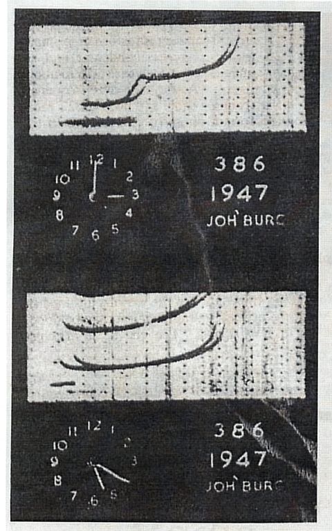
Fig 6. Two images from the long-afterglow tube taken on June 1947 (given in 'half-day' units) during the mid- and late afternoon. The frequency and height markers are clearly evident. The upper trace shows the interesting sporadic E phenomenon at 100km, as well as the F1 and F2 layers higher up.
Several of these ionosondes were subsequently manufacturcd by the TRL. One was operated from the TRL laboratories in Johannesburg before being moved some distance from the city to a quieter site, while the other was situated near Cape Town. Once set up neither piece of equipment required any maintenance other than the need to replace the occasional valve every few months. The reasons for valve failure were invariably due to open-circuited cathodes caused by the switching cycle on the filaments. Wadley believed that it was preferable for valves to fail for that reason rather than due to loss of emission as would have happened had the filament been energised continuously. The only routine activity involved the removal of 12 feet of film once a week.
Antenna
Though the published details are sparse a brief comment about the antenna used with the ionosonde is of interest. According to Wadley's published paper, the antenna consisted of two, concentric vertical rhombics that were switched between transmitter and receiver. Their centre frequencies were quoted as 4 and 12MHz respectively and so, together, they covered the required band fairly effectively. Each rhombic was connected to an air-cored transformer whose secondaries were very tightly coupled.
Correct phasing of the antenna currents was achieved by reversing one of the transmission lines, if necessary. The transformers were then fed in push-pull by the transmitter at an impedancc of about 1000 ohms. One must assume, for purely practical reasons, that the antennas, though rhombic in shape, were by no means the size of the classic rhombics at the lower frequencies since true rhombics at the lower frequencies have leg lengths typically many wavelengths per side. It is reported that the wooden lattice mast that supported the antennas when the ionosonde was moved out of the centre of Johannesburg was 60m in height. True rhombic performance would have occurred at frequencies above about 12 MHz but below that the radiation pattern will have broadened considerably.
Though modified occasionally to upgrade some of their features, Wadley's two ionosondes remained in service for more than twenty years. They provided data from which the NITR (National Institute for Telecommunications Research), the TRL's successor, generated a monthly series of HF predictions that served the communications needs of many southern African states. In conjunction with a more recent ionosonde installed at Rhodes University in Grahamstown, as well as occasional ionospheric soundings carried out from South Africa's Antarctic base and its south Atlantic islands, those instruments provided vitally important data from the southern tip of a vast continent, not well-served by such facilities, to the world databank maintained by the international ionospheric research community.
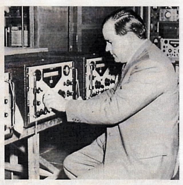
Fig. 7. Trevor Wadley seated in front of a bank of the famous RA17 receivers that were based
on ideas developed for his Ionosonde.
Conclusion
Trevor Wadley's genius was soon recognised on a much wider stage. In 1954 his continuously tunable HF receiver, which followed directly from his ionosonde, became the RA17 when manufactured by Racal in Bracknell. For many years it remained the most successful communications receiver in use anywhere in the world. In that same year he designed a revolutionary microwave-surveying instrument that measured distance to an accuracy of one in a hundred thousand, a figure unheard of at that time. It went into production as the Tellurometer in 1957.
Acknowledgements
Acknowledgement is made to the IEE (now the IET) for permission to publish the photographs of the ionosonde and to the Rutherford Appleton Laboratory for use of the ionogram and the photograph of the original Slough transmitter.
Bibliography
T L Wadley, A Single-Band 0 - 20Mc/s Ionosphere Recorder embodying some new techniques, Proc IEE, Vol.96, Pt.III, 1949, pp 483-486.
H. Rishbeth, C J Davis, The 70th anniversary of ionospheric sounding, Engineering Science and Education Journal (IEE), Vol. 10, issue 4, 2001, pp 139-144.
K R Thrower, Racal and the RA.17 HF Communications Receiver, parts 1 and 2, Radio Bygones, Nos.25 and 26, 1993, pp.4-9; 17-26.
O. G. Villard, The ionospheric sounder and its place in the history of radio science, Radio Science, Vol. II, no.l1, 1976, pp.847-860.
D. G. Kingwill, The CSIR - the first 40 years, (CSIR, Pretoria) 1990, Pt.3 Telecommunications and Radiophysics, pp.174-180.
D C Baker, Ionosonde Stations in Southern Africa - a review of current status and future prospects, Ionosphere Network Advisory Group INAG, UAG-I04, (1993), http://www.ips.gov.au/IPS Hosted/IN AG/uag-104/text/baker.html.
Return to Journal Index OR Society's Home page
South African Military History Society / scribe@samilitaryhistory.org